After reading this article you will learn about the estimation of similarities between two individual taxa.
The similarity data is used to estimate distance between two individual taxa.
The illustrated example taken from Henry (1997) is as follows:
Let us say we have data from RAPD results for 2 samples A and B. Similarity (F) can be calculated as
Similarity (F) = 2(nxy)/nx + ny
Where nxy = number of bands in common to sample A and sample B
nx = number of bands for sample A
ny = number of bands for sample B
If sample A and B both had a total of 100 bands each as a result of amplification and there were 75 common bands, then
F = 2 x 75/100 + 100 = 0.75 (75% similarity)
The above equation has been proposed by Nei and Li (1979).
The alternative formula known as Jaccard’s coefficient is as follows:
F’ = nxy / (nt – nz)
Where nxy = number of bands in common to sample A and sample B
nt = total number of bands present in all samples
nz = number of bands not present in sample A or B but found in other samples
In the example as given above, if other samples contributed to give a total of 200 bands amplified with 75 of them being absent in both A and B, the Jaccard coefficient
F’ = 75/200 – 75 = 0.66
F may also be calculated through other formulae, like
F’’ = (nxy + nx)/nt
F’’’ = nz/(nt – nxy)
Dissimilarity the inverse of similarity is normally 1- F. A distance matrix of dissimilarity or dissimilarity can be prepared for any set of individuals. If a third sample C (also resulting in 100 bands, 50 in common with sample A and 60 in common with sample B) is considered.
The data could be presented in the following dissimilarity matrix:
For illustration, using the formula of Nei and Li, a few similarity coefficients can be calculated as:
Similarity between A and B = 2 x . 75/100 + 100 = 0.75 and
Dissimilarity = 1-0.75 = 0.25
Similarity between A and C = 2 X 50/100 + 100 = 0.50 and
Dissimilarity = 1-0.50 = 0.50
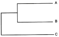
Using the dissimilarity coefficient from the above matrix, a phenogram can be generated using an un-weighted pair group method with arithmetic mean analysis (UPGMA) as follows. If we consider the closest pair of samples A and B as a cluster as their dissimilarity coefficient was the least (0.25) in the matrix given above, then the average distance of A and B from a common ancestor can be considered to be 0.25/2 = 0.125.
Now A and B can be considered as a single entity AB.
The dissimilarity of AB from C (the next closest sample) is now computed as the average of the dissimilarities from A and B as given below:
0.50 + 0.40/2 = 0.45
In the cluster of C and AB, the average distance of C and AB from a common ancestor can be considered to be as:
0.45/2 = 0.225
From these average distances, the phenogram of A, B and C can be illustrated as follows:
0.25 0.20 0.15 0.10 0.05 (1 – F)
This illustration is much simpler as only 3 samples were involved. In case of large number of genotypes which often is the case, phenograms are constructed using computer software using the UPGMA. Some of the computer software are NT-SYS, PHYLIP, PAUP and MacClade.

