After reading this article you will learn about:- 1. Detection of Linkage Using F2 Data 2. Detection of Linkage Using Backcross (Testcross) Data.
Detection of Linkage Using F2 Data:
It may be recalled that when 2 genes are located on 2 different chromosomes, they assort independently and give rise to a typical 9:3:3:1 ratio in the F2 generation assuming complete dominance at both the loci. Under this situation, typical backcross (testcross) ratio is 1 : 1 : 1: 1. Failure of fulfillment of these ratios is an indication of abnormal segregation at either loci or involvement of linkage.
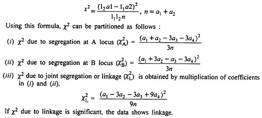
When an F2 data fails to conform to a 9 : 3 : 3 : 1 ratio as revealed by χ2 test, the χ2 is partitioned into various components to confirm if linkage is involved as explained below:
When only 2 classes al and a2 are available in a ratio of 11 : 12, χ2 can be calculated using direct values also using the formula:
Numerical Illustration:
χ2T = 4.17 + 8.00 + 5.56 + 8.17 = 25.90
χ2T with a value of 25.90 is highly significant at 3 degrees of freedom indicating non- fulfillment of 9 : 3 : 3 : 1 ratio.
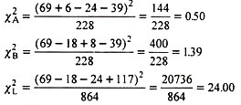
Hence, this χ2 value is partitioned into components as:
Each of above 3 χ2 values has 1 degree of freedom. Calculated χA2 is not significant showing normal segregation at A locus. Similar is the case at B locus. However, χL2 is significant clearly showing that significant departure from 9: 3: 3: 1 F2 ratio in the original data can be ascribed to linkage.
Detection of Linkage Using Backcross (Testcross) Data:
Numerical Illustration:
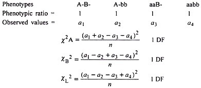
The backcross (testcross) data is tested for goodness of fit for the expected ratio 1:1:1:1. In the event of failure of this hypothesis, the resultant χ2 is partitioned as given above, for example:
The data clearly shows that it does not fit to 1: 1: 1: 1 ratio. Further after partitioning of X2 (33.84), into XA2, XB2 and XL2, the linkage is apparent.
The formulae as given above for F2 and backcross data are valid for coupling phase (both the dominant genes in one parent and both the recessive genes in another parent).
The same formulae are applicable to repulsion phase data (AAbb x aaBB) also but the classes are inverted as:


