After reading this article we will learn about the Hardy-Weinberg equilibrium of gene.
In a large random mating population, both gene and genotype frequencies remain constant from generation to generation, in absence of migration, mutation and selection. These properties of a population were first demonstrated by Hardy and Weinberg independently in 1908, and are generally known as Hardy-Weinberg law. If A = p and a = q, after random mating among gametes.
The resultant population will be as follows:
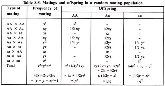
Thus a population in Hardy-Weinberg equilibrium has the gene and genotype frequencies as p : q and p2 : 2 pq : q2 respectively. These genotype frequencies are established after 1 generation of random mating irrespective of the initial genotype frequencies among the parents. This is illustrated by random mating among 3 genotypes, AA, Aa, aa.
The consequences of this random mating are summarised in Table 8.8.
Thus, x, y, z frequencies of genotypes AA, Aa, aa respectively become in an equilibrium proportion of p2 : 2pq : q2 after 1 generation of random mating.
The gene frequencies in the population obtained 1 generation of random mating are as:
P1 = p2 + 1/2 (2pq)
= p2 + pq
= p (p + q) = p, (p + q= 1)
i.e. it is the same as that which existed in the original population.
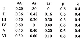
The population with identical gene frequencies may not necessarily have similar genotype frequencies as illustrated below:
Although all the 6 populations as above have different genotypic frequencies, they all will reach to an equilibrium state of p2 : 2 pq : q2 (0.36 : 0.48 : .16) after 1 generation of random mating and population II is already in this state from the beginning itself.
When a character is governed by a recessive gene, genotypic frequencies at equilibrium can be calculated easily as:
Multiple Alleles:
Hardy-Weinberg equilibrium is easily extendable to multiple allelic situations.
If there are 3 alleles, A1, A2, A3 with frequencies of p, q and r respectively where p + q + r = 1 then various genotypes in a population in equilibrium shall be as follows:
p2 + 2pq + 2pr + q2 + 2qr + r2 is straight away square of gametic gene frequencies, i.e. = (p + q + r)2
Multiple Loci and Genetic Equilibrium:
Let us consider 2 loci A and B with gene frequencies as:
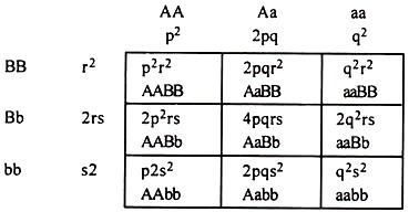
Mono-factorial genotype frequencies at equilibrium will be:
At A locus – P2 (AA) : 2pq (Aa) : q2 (aa)
At B locus – r2 (BB) : 2rs (Bb) : s2 (bb)
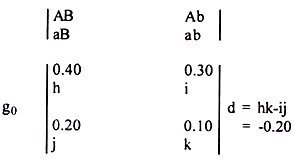
The bi-factorial gametes will be as:
At equilibrium h = pr, i = ps, J = qr and k = qs and which further leads to hk = ij. That means if the equilibrium prevails, the frequency of each sort of gamete is given by the product of frequencies of alleles contained therein.
For example,
Thus, the given population is not in equilibrium with respect to these alleles as h ≠ pr and so on.
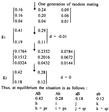
At equilibrium the gamete frequencies will be:
The relationship that frequency of gamete AB is h = pr etc. can be demonstrated as follows:
The same is true for other gametes.
Consequently, at equilibrium,
h = pr, i = ps, j = qr, k = qs and hk = ij
Numerical Illustration:
This way the population approaches to equilibrium gradually, where ‘d’ is halved in each generation of random mating till it becomes zero. However, for individual locus it reaches to equilibrium only after 1 generation of random mating.

