The below mentioned article provides a study note on chi-square test.
In biological experiments and field surveys, apart from quantitative data we get the qualitative data which is genetical character such as tall and short, colour of flower, seed coat character which do not have any numerical values. But the number of flowers or seeds having a particular colour falls under any category can be counted numerically.
This type of observation requires the calculation of the expected number of individuals under any category. Thus it becomes necessary to know whether there is any deviation in between the observed and expected frequencies. The measurement of this deviation is done with the help of a particular test which is called Chi-square (X2) test.
The formula for Chi-square test is:
X2 = ∑(O-E)2/E
where O = Observed value,
E = Expected value.
Application of X2-Test:
It is an alternative test to find significance of difference in two or more than two proportions:
(a) It can compare the values of two binomial samples when they are small.
(b) It can compare the frequencies of two multinomial samples.
(c) Chi-square measures the probability of association between two discrete attributes.
(d) The Chi-square test is applied as a test for goodness of fit which reveals the closeliness of observed frequency with those of the expected frequency. Thus it helps to answer whether physical or chemical factors did or did not have an effect.
(e) Occasionally it is desirable to compare one set of observations taken under particular conditions to those of a similar nature taken under different conditions. In this case there are no definite expected values, only the question is whether the results are dependent (contingent upon) or independent of conditions. Then the X2-test is called as test for independence or contingency test.
X2-Test For Goodness of Fit:
X2-test is applied to a wide range of studies relating to experimental biology and field studies. The aim of this test is to test the closeliness of observed frequencies with those of the expected, i.e., how well the observed frequency curve fits into theoretical curve.
If both the observed and expected frequency distribution are in complete agreement with each other then the X2-value will be zero. But in experimental observations there is always some degree of deviation. The critical X2-value will be exceeded due to sampling fluctuations.
For example, if a crossing experiment gives two different sizes of seeds in F2 progeny then these two types seeds may segregate according to 3:1 (Mendelian Monohybrid), 1:1 (Monohybrid test cross), 9:7 (Complementary factor interaction), 13:3 (Inhibitory factor) or 15:1 (Duplicate gene interaction) ratio, etc.
Again if crossing experiment results in three types of seeds then these may be due to incomplete dominance (1:2:1), supplementary factor (9:3:4) or due to dominant epistasis (12:3:1) interaction, etc.
Likely, 4 types of seeds with 4 different combinations of two different characters may either follow the 9:3:3:1 (Mendelian dihybrid) or 1:1:1:1 (Dihybrid test cross) ratio for segregation.
Test for the goodness of fit is required in these above cases for studying the closeliness of observed data of the experiments with those of expected frequencies.
Steps to be followed to test the Goodness of Fit:
1. Deviation between the observed and the expected results should be calculated.
2. Comparing the minimum deviation the null hypothesis should be selected for X2-test.
3. X2-value should be determined.
4. Comparing the calculated X2-value with tabulated X2-value the conclusion has to be made.
Example 7 → (3:1):
Following number of seeds with the associated character is observed. Test the goodness of fit and comment.
Yellow seed: 428
Green seed: 152
Step I: Calculation of expected value for each ratio:
Step II: Determination of expected segregation ratio:
According to table, the deviation is minimum in 3:1 ratio, so the observed sample should fit the 3:1 ratio.
Step-III Calculation of X2-Value:
Since, in this experiment the samples are of two classes, so degree of freedom = 2-1 = 1.
Step IV: Conclusion:
The calculated Chi-square (X2) value is 0.451. The tabulated chi-square at 0.05 probability level with 1 degree of freedom is 3.841.
The calculated value is much less than the table value, so the deviation is insignificant, the observed deviation is due to chance factor only. It lies in the probability range 50-70%.
The observed result is in good fit with Mendelian Monohybrid ratio, i.e., 3:1.
Step V: Comment:
Comment:
It is concluded that the experimental result shows Mendelian monohybrid ratio 3:1.
So the assumed genotypes of parents are:
So the phenotypic ratio is 3:1.
Example 8 → (9:3:3:1):
In an experiment on garden pea, we count 4 different kinds of plants,
Test the goodness of fit for this data and comment.
Step I: Calculation of expected value of assumed ratio:
Since, in this experiment the samples are of 4 classes, so degrees of freedom = 4-1
Step IV: Conclusion:
The tabulated X2 value at 0.05 probability level for 3 degree of freedom is 7.81 which is more than the calculated value and it lies at 90-95% probability level. So the deviation found in the experiment is insignificant.
We can conclude that the observation is in good fit with Mendelian Dihybrid ratio 9:3:3:1.
Step V: Comment:
As the observation shows good fit with Mendelian dihybrid ratio, so the two genes for cotyledon colour and pod shape can independently assort.
Example 9 → (1:1):
One yellow seeded pea plant when crossed with a green seeded pea plant, produced 50 yellow seeds and 46 green seeds in F2. Write down your comment with the help of x2-analysis.
Sample character and sample size
According to the table, we find that the minimum deviation is in case of 1:1 ratio. So it is assumed that the observed sample should fit well with this ratio.
Conclusion:
Since there are 2 classes, so the degree of freedom = 2-1 = 1. The calculated X2-value is 0.166 which is much less than the table value 3.841 for 1 degree of freedom at 0.05 probability levels.
The X2 value 0.166 lies between 80-90% probability level. Therefore the deviation which is observed in the sample from the expected value is highly insignificant, and the observed ratio has a very good fit with the expected ratio, i.e., 1:1.
Comment:
As the experimental result shows good fit with 1:1 ratio, i.e., Mendelian monohybrid test cross ratio, so the assumed genotypes of the parents and the offsprings are as follows:
Example 10→(9:7):
Selfing of a hybrid plant produced a population with 120 pink flowers and 88 white flowers. Explain with X2-analysis, what does the result show?
According to this table, we find that the deviation is minimum in case of 9:7 ratio. So, it is assumed that the observation should fit well with this ratio.
Conclusion:
Since in the observation there are two classes, so the degree of freedom =2 – 1 = 1
The calculated X2 value is 0.175, which is much less than the table value 3.84 for 1 degree of freedom at 0.05 probability level.
The X2 value 0.175 lies between 50-70% probability range. Therefore this deviation from the expected value is insignificant and the observed ratio is in good fit with 9:7 ratio.
Comment:
It is concluded that the experimental result shows the characters with complementary factor interaction in F2 generation.
As the observed samples are assumed to show complementary factor interaction, so the assumed genotypes are:
Here, the analysis shows that 2 pairs of factors control the same character and two dominant genes A and B are complementary to each other. Each of which has no effect on expression of character, but when in combination shows their effect, i.e., pink colour.
Absence of any one of the them (A or B) leads to absence of pink colour and it can be concluded very easily that the colour character is controlled by two pairs of factors which are complementary to each other.
Example 11 → (13:3):
From a plant after selfing total 96 seeds are harvested of which yellow seeds 79, brown seeds 17. Explain the result with X2-analysis.
Sample character and sample size
Determination of expected segregation ratio:
(By estimating magnitude of deviation)
According to the table, we find that the minimum deviation is in case of 13:3 ratio. So it is assumed that the observed sample should fit well with this ratio.
Determination of Chi-Square value
Conclusion:
Since there are two classes, degree of freedom = 2-1 = 1. The calculated X2 value 0.068 is much less than the table value 3.841 for 1 degree of freedom at 0.05 probability level.
The X2-value 0.068 lies between 90-95% probability level. Therefore, this deviation from the expected value is highly insignificant and the observed ratio has a very good fit with the expected ratio.
Comment:
As the experimental result shows good fit with 13:3 ratio. So it is assumed that the brown colour of seed coat is controlled by gene C, but the presence of another dominant gene D inhibits the effect of C, and the seed coat colour becomes yellow.
The dominant gene D does not have its own expression but it inhibits the effect of another dominant gene C. So the effect of C is only expressed when there is recessive gene d. This phenomenon is called Inhibitory Factor.
So, the phenotypic ratio of Yellow seed: Brown seed = 13: 3.
Example 12 → 15:1):
In an experiment, the hybrid plant yielded 193 brown coloured seeds and 15 white seeds. Comment on the observed result with X2-analysis.
Sample character and sample size:
Determination o expected segregation ration:
(By estimating magnitude of deviation)
According to the table, we find that the deviation is minimum in case of 15:1 ratio. So, it is assumed that the observed sample should fit with this ratio.
Determination of Chi-square value
Conclusion:
Since there are two classes, degree of freedom = 2 – 1 = 1. The calculated X2 value 0.332 is less than the table value 3.841 for 1 degree of freedom at 0.05 probability level.
The X2 value 0.332 lies between 75-90% probability levels. Therefore this deviation from the expected value is insignificant and the observed ratio has good fit with the expected ratio.
Comment:
As the experimental result shows good fit with 15:1 ratio, so it is assumed that the brown colour of seed is controlled by two pairs of factors or alleles. Presence of any one of them will give them brown seed colour. Whereas the recessive condition of both will give the white colour.
This case may be represented as follows:
So the observed result shows the duplicate factor interaction in F2 ratio.
Example 13 → (1:1:1:1):
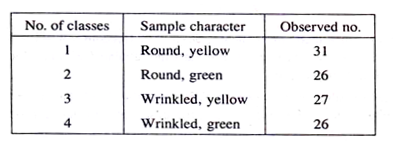
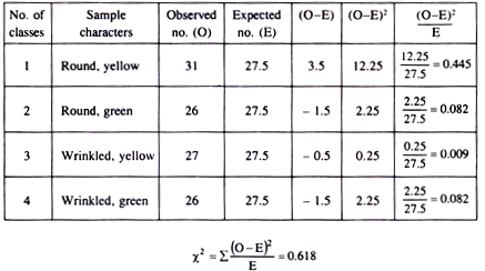
Test the goodness of fit in the following sample from an experiment with garden pea plant.
Round, yellow 31
Round, green 26
Wrinkled, yellow 27
Wrinkled, green 26
Determination of expected segregation ratio:
According to the table, we find that the deviation is minimum in case of 1:1:1:1 ratio. So, it is assumed that the observed sample should fit with this ratio.
Determination of Chi-square value
Conclusion:
Since there are 4 classes, degrees of freedom = 4-1=3. The calculated X2 value is 0.618, which is much less than the tabulated X2 value for 3 degree of freedom at 0.05 probability level.
The calculated value lies between 70-90% probability level. Therefore the deviation from the expected value is insignificant and the observed ratio has a good fit with the expected ratio.
Comment:
As the experimental result shows good fit with 1:1:1:1 ratio, so it is assumed that the result is obtained from a dihybrid test cross. The dominant characters are yellow and round.
Parental genotypes are assumed as:
Example 14→ (An example not in agreement with 1:2:1):
A geneticist obtained 209 plants after selfing a hybrid, among which with red flower = 52 plants, with pink flower = 128 plants and with white flower = 29 plants. Show the goodness of fit with 1:2:1 ratio.
Determination of expected frequency of different plant:
Calculation of Chi-square value:
Conclusion:
The calculated value of X2 = 15.626. Since there are 3 classes, so the degrees of freedom = (3 – 1) = 2. The tabulated X2 value for 2 degree of freedom at 0.05 probability level is 5.99. As the observed value is much higher than the tabulated value, so the result does not in agreement with 1:2:1 ratio, i.e., the observation does not show goodness of fit with the expected ratio.
In conclusion, the principle of incomplete dominance is not applicable here.
Chi-Square Test for Association Of Attributes:
By using 2×2 contingency table the X2 analysis is applied to test whether there is any association between two or more classifications, i.e., to test for independence of the two attributes.
Steps to be followed to calculate Chi-Square:
1. Null hypothesis should be set up, which is no association exists between the attributes.
H0: No association exists between the attributes.
H1 : Association exists between the attributes.
2. Expected frequency (E) is calculated corresponding to each category by the formula.
Eij = Ri × Cj/n
Ri = Sum total of row in which Eij is present.
Cj = Sum total of column in which Eij is present,
n = Total sample.
3. The Chi-square value is calculated according to formula
Degrees of freedom = (R – 1) (C – 1)
R = No. of rows,
C = No. of columns.
4. Table value is found out for a particular level of significance and for the calculated degree of freedom.
5. The calculated value and table value are compared, if the calculated value of X2 < the table value then the null hypothesis is accepted. But if the X2 value is larger than the tabulated value then null hypothesis is rejected.
Example 15:
An experiment was carried out to see the effect of an organo-mercuric compound on the survival of seedling. Two different concentrations are applied to test whether the percentage of death in higher concentration is significantly different from that of lower concentration or both are independent.
In this case the null hypothesis will be – there is no significant difference, i.e., both the effects are independent.
H0: Both the effects are independent.
H1: Both the effects are significantly different.
Table showing expected results and deviation
In this example, as the (O-E) is always 5.2, so we can compute the value in following way.
The degree of freedom for this example is
(C-1XR-1) = (2-1) x (2-1) = 1
The tabulated X2 value at degree of freedom 1, and at p = 0.05 level is 3.84.
As the calculated X2 value is much less than the tabulated X2 value so the null hypothesis is accepted, i.e., both the effects are independent, there is no relation of death percentage with low and high concentration of fungicide.
Yates Correction:
Yates correction is applied to increase the precision of X2 test, only when the degree of freedom is 1 and the expected classes are small (less than 30). In case of 1 degree of freedom, there is possibility of underestimating the probabilities listed in the table. This can be adjusted by subtracting the correction value from the deviation value.
For goodness of fit, Chi-square formula using Yates correction (½ or 0.5) will be:
In Example 12,
In case of contingency Chi-square, using Yates correction the Chi-square value is calculated as follows:
If we apply this formula in the Example 15, then


